 Image credit: Unsplash
Time Series Forecasting using Facebook Prophet
Forecasting with time series models can be used by businesses for many purposes, for example, to optimise sales, improve supply chain planning and many other. There are many different techniques you can use solve such problems.
In this article we’ll use Prophet, a open-source package developed by Facebook to perform time series forecasting.
Introduction
Prophet is an open-source package for univariate (one variable) time series forecasting developed by Facebook.
Prophet implements additive time series forecasting model, and the implementation supports trends, seasonality, and holidays. This package provides two interfaces, including R and Python. We will focus on the Python interface.
Installation
Prophet can be installed using either command prompt or Anaconda prompt using pip as shown below. Prophet depends on a Python module called pystan.
pip install fbprophet
Now we have Prophet installed, let’s select a dataset we can use to explore using the package.
Avocado Dataset
We will use the Avocado dataset. The data set includes information about the prices of (Hass) avocados and the amount sold (of different kinds) at different points in time.
Columns of interest are:
Date: date of the observationAveragePrice: average price of a single avocadoTotal Volume: total number of avocados soldtype: whether the price/amount is for conventional or organic4046: total number of small avocados sold (PLU 4046)4225: total number of medium avocados sold (PLU 4225)4770: total number of large avocados sold (PLU 4770)Region: the city or region of the observation
Let’s load and explore the dataset.
Import Packages
Import required packages:
import numpy as np
import pandas as pd
from fbprophet import Prophet
Loading dataset
df = pd.read_csv("data/avocado.csv")
df.head(2)
| Unnamed: 0 | Date | AveragePrice | Total Volume | 4046 | 4225 | 4770 | Total Bags | Small Bags | Large Bags | XLarge Bags | type | year | region |
|---|---|---|---|---|---|---|---|---|---|---|---|---|---|
| 0 | 2015-12-27 | 1.33 | 64236.62 | 1036.74 | 54454.85 | 48.16 | 8696.87 | 8603.62 | 93.25 | 0.0 | conventional | 2015 | Albany |
| 1 | 2015-12-20 | 1.35 | 54876.98 | 674.28 | 44638.81 | 58.33 | 9505.56 | 9408.07 | 97.49 | 0.0 | conventional | 2015 | Albany |
For simplicity, we’ll only select the AveragePrice prices for conventional avocodos from dataset
df_avocado = df[(df.type == 'conventional') ]
df_avocado['Date'] = pd.to_datetime(df_avocado['Date'])
df_avocado = df_avocado.sort_values("Date")
Dataset for Prophet
Prophet is expecting columns to have specific names, ds for the temporal part and y for the value part. We’ll prepare data according to that.
df_avocado = df_avocado[['Date', 'AveragePrice']].reset_index(drop=True)
df_avocado.rename(columns={'Date':'ds', 'AveragePrice':'y'}, inplace=True)
df_avocado.head(2)
| ds | y | |
|---|---|---|
| 0 | 2015-01-04 | 0.93 |
| 1 | 2015-01-04 | 1.10 |
It’s always a good idea to plot the data to get a first impression on what we are dealing with. We’ll plot.ly for plotting charts.
import plotly.express as px

fig = px.line(df_avocado, x='ds', y='y', title='Line Plot of Avocado Dataset')
fig.show()
We can see the trend in average price over time. Such patterns we expect the forecast model should consider.
Now we are familiar with the dataset, let’s explore how we can make a use of the Prophet package to make forecasts.
Forecast avocodos average price with Prophet
Let’s start by fitting a model on the dataset
Fit Prophet model
Now let’s create the Prophet instance with all default values, fit the dataset.
m = Prophet()
m.fit(df_avocado)
Make future prediction
For predicting the values using Prophet, we need to create a dataframe containing the dates for which we want to make the predictions.
We’ll use make_future_dataframe() to specify the number of days to extend into the future. By default it includes dates from the history.
future = m.make_future_dataframe(periods=365)
future.tail(2)
| ds | |
|---|---|
| 532 | 2019-03-24 |
| 533 | 2019-03-25 |
Now, Create the forecast object which will hold all of the resulting data from the forecast.
forecast = m.predict(future)
When listing the forecast dataframe we get:
forecast.head(2)
| ds | yhat_lower | yhat_upper | yhat | |
|---|---|---|---|---|
| 0 | 2015-01-04 | 0.805868 | 1.368417 | 1.103528 |
| 1 | 2015-01-11 | 0.864619 | 1.381266 | 1.117847 |
The yhat contains the predictions and then you have lower and upper bands of the predictions.
Plotting forecast data
Here, Prophet provides convenience methods for plotting.
### Simple plot
# fig = m.plot(forecast)

### Using plot.ly
from fbprophet.plot import plot_plotly

plot_plotly(m, forecast)
You can also add change-points (where the trend model is shifting) to the plot like this:
### Simple plot

# from fbprophet.plot import add_changepoints_to_plot

# fig = m.plot(forecast)
# a = add_changepoints_to_plot(fig.gca(), m, forecast)

### Using plot.ly
from fbprophet.plot import plot_plotly

plot_plotly(m, forecast, changepoints=True)
Plotting the forecasted components
We can also plot all the components that make up the model: trend, seasonality
from fbprophet.plot import plot_components_plotly

### Using plot.ly
plot_components_plotly(m, forecast)

### simple plot
# fig = m.plot_components(forecast)
Prophet learns that price is usually going up from July to December.
Cross Validaton
In order for us to find out how our model performs and know if we are making progress we need some kind of validation. Prophet includes functionality for time series cross validation to measure forecast error using historical data.
This cross validation procedure can be done automatically for a range of historical cutoffs using the cross_validation function. We specify,
horizon- the forecast horizoninitial- the size of the initial training periodperiod- the spacing between cutoff dates
By default, the initial training period is set to three times the horizon, and cutoffs (period) are made every half a horizon.
The resulting dataframe can now be used to compute error measures of yhat vs. y.
Here we do cross-validation to assess prediction performance on a horizon of 180 days, starting with 540 days of training data in the first cutoff and then making predictions every 31 days.
You can read more on Prophet Cross Validation here.
from fbprophet.diagnostics import cross_validation

df_cv = cross_validation(m, initial='540 days', period='31 days', horizon = '180 days')
Performance Metrics
Prophet comes with some built-in performance metrics, The performance metrics available are:
mse: mean absolute errorrmse: mean squared errormae: Mean average errormape: Mean average percentage errormdape: Median average percentage error
The code for validating and gathering performance metrics is shown below:
from fbprophet.diagnostics import performance_metrics
df_p = performance_metrics(df_cv)
df_p.head(2)
| horizon | mse | rmse | mae | mape | mdape | coverage | |
|---|---|---|---|---|---|---|---|
| 0 | 19 days | 0.077039 | 0.277560 | 0.224990 | 0.191728 | 0.147702 | 0.601132 |
| 1 | 20 days | 0.077200 | 0.277849 | 0.225041 | 0.191624 | 0.146887 | 0.602669 |
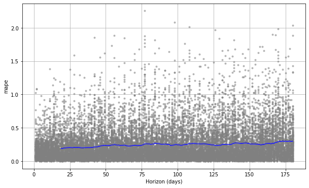
Cross validation performance metrics can be visualized with plot_cross_validation_metric, here shown for MAPE. Dots show the absolute percent error for each prediction in df_cv. The blue line shows the MAPE.
It shows that errors around 20% are typical for predictions 20 days into the future, and that errors increase up to around 30% for predictions 180 days into the future.
from fbprophet.plot import plot_cross_validation_metric

fig = plot_cross_validation_metric(df_cv, metric='mape')

Improvements
You can further improve your models by adding holidays, adding extra regressors and by tuning hyperparameters. Learn more from here.
Saving/Loading Prophet models
Here Prophet provides the built-in serialization functions to serialize the model to json:
import json
from fbprophet.serialize import model_to_json, model_from_json

with open('models/model_avocados_avg_prices.json', 'w') as fout:
    json.dump(model_to_json(m), fout)  # Save model

with open('models/model_avocados_avg_prices.json', 'r') as fin:
    m = model_from_json(json.load(fin))  # Load model
Conclusion
In this article, you have learned how to use the Facebook Prophet package to make time series forecasts. We have learned how to fit the model over dataset and make future predictions, plot the results, validate and look at the performance metrics.
I hope this article was valuable to you and that you learned something that you can use in your own work.
Go ahead and clone the repos time-series-prophet to view the full code of the project.
Happy Forecasting!
Releted Posts
Improving Business Processes using Machine Learning
Imagine your business has a contact form on its website. Every day you get many messages from the form, many of which are actionable, but it’s easy to fall behind on dealing with them since different employees handle different queries.
Read moreSentiment Analysis on Earnings Call Transcript
Earning call is a conference call between executives and major investors where they discuss their quarterly financial performance and future outlook.
Read moreBuild a CRUD App in React
In this article, We’ll walk step-by-step through the process of building out a simple React CRUD app with Web API. It will have tasks, we’ll be able to add, update, list or delete tasks.
Read more

